Public Health
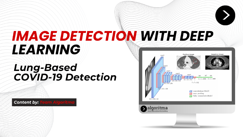
Lung-Based COVID-19 Detection
Background
“It is better to light a candle than curse the darkness."
Nowadays, every country in a corner of the world is still surviving about COVID-19. COVID-19, the worldwide-pandemic, is an issue that need to be highly concerned by everyone. Based on WHO’s data, ’till March 2021, the number of COVID-19’s survivor in the world is around 127 million people. Wow, it’s a very high number, right?!
Like the quote above, we better to light a candle than curse the darkness. Using the power of technology and especially artificial intelligence, we can light the candle in this darkness because of COVID-19 pandemic. Yay!
Because of this virus is a new virus and didn’t exist before, the researchers is still investigate the symptomps and the affect of COVID-19 to help the health-sector provide the best action to handle this virus. Based on theconversation.com, lungs are the organ most commonly affected by COVID-19, with a spectrum of severe effects. Because of COVID-19, people can have pneumonia, acute respiratory distress syndrome (ARDS), and other respiratory syndrome. Compared to other respiratory viruses, it causes marked clotting in the small blood vessels of the lungs.
So, in this case we want to detect COVID-19 on the human’s body by using Lung CT Scan-Images.
Data Preparation
Data that used on this case is images from https://www.kaggle.com/luisblanche/covidct. The images are collected from COVID19-related papers from medRxiv, bioRxiv, NEJM, JAMA, Lancet, etc. CTs containing COVID-19 abnormalities are selected by reading the figure captions in the papers.
We will use Python to processing our data and build the model
Import Library
First of all, we need to import library and package that needed on our next modeling
Import Data
And then, we import the data that we’ve already downloaded before. Because of our data is images, we use some library like os and glob to connecting and joining our images data.
We have 2 categories of images, lung of image from COVID-19 survivor and not.
1
2
3
|
data_root='dataset'
path_positive_covid = os.path.join(data_root, 'CT_COVID')
path_negative_covid = os.path.join(data_root, 'CT_NonCOVID')
|
1
2
|
# Print the paths to verify them
print(f"Path to positive COVID images: {path_positive_covid}")
|
1
|
#> Path to positive COVID images: dataset\CT_COVID
|
1
|
print(f"Path to negative COVID images: {path_negative_covid}")
|
1
|
#> Path to negative COVID images: dataset\CT_NonCOVID
|
1
2
3
4
|
# Collecting image file paths
positive_images = glob(os.path.join(path_positive_covid, "*.png"))
negative_images = glob(os.path.join(path_negative_covid, "*.png"))
negative_images.extend(glob(os.path.join(path_negative_covid, "*.jpg")))
|
 1
 2
 3
 4
 5
 6
 7
 8
 9
10
11
|
covid = {
    'class': 'CT_COVID',
    'path': path_positive_covid,
    'images': positive_images
}

non_covid = {
    'class': 'CT_NonCOVID',
    'path': path_negative_covid,
    'images': negative_images
}
|
Exploratory Data Analysis
We can check our data detail to make sure that we already import the data properly.
 1
 2
 3
 4
 5
 6
 7
 8
 9
10
11
12
13
14
15
16
17
18
19
20
21
22
23
24
25
26
27
28
29
30
31
|
if positive_images and negative_images:
try:
# Read the images
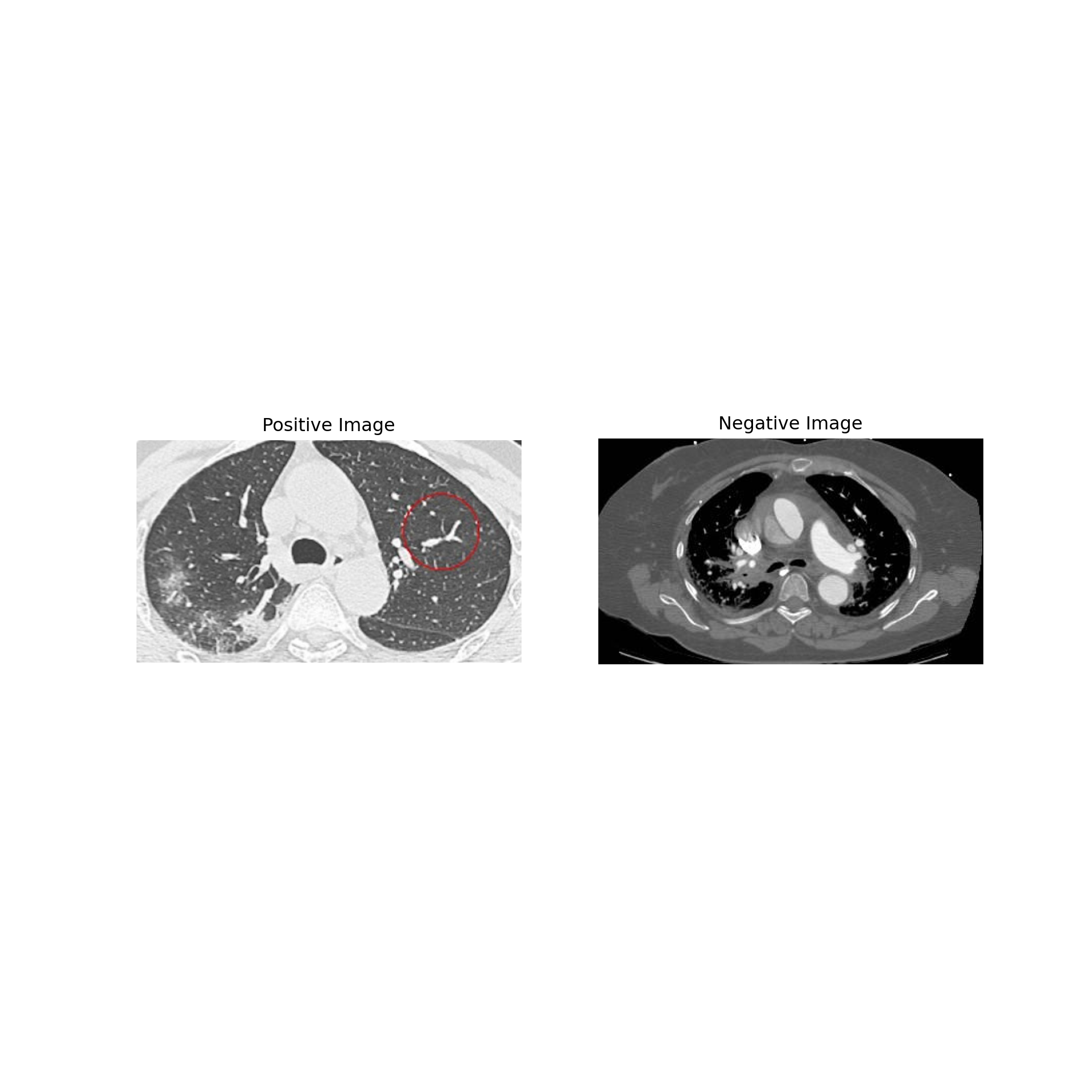
ex_positive = cv2.imread(positive_images[0])
ex_negative = cv2.imread(negative_images[0])
# Check if the images are loaded correctly
if ex_positive is not None and ex_negative is not None:
# Convert images from BGR to RGB (OpenCV loads images in BGR format)
ex_positive = cv2.cvtColor(ex_positive, cv2.COLOR_BGR2RGB)
ex_negative = cv2.cvtColor(ex_negative, cv2.COLOR_BGR2RGB)
# Create the plot
fig = plt.figure(figsize=(10, 10))
ax1 = fig.add_subplot(1, 2, 1)
ax1.imshow(ex_positive)
ax1.set_title('Positive Image')
ax1.axis('off')
ax2 = fig.add_subplot(1, 2, 2)
ax2.imshow(ex_negative)
ax2.set_title('Negative Image')
ax2.axis('off')
plt.show() # Display the plot
else:
print("Error: One of the images couldn't be loaded. Check the file paths.")
except Exception as e:
print(f"An error occurred: {e}")
else:
print("Error: Image lists are empty. Please provide valid image paths.")
|
1
2
3
4
5
6
|
#> <matplotlib.image.AxesImage object at 0x000001E0DAAA5ED0>
#> Text(0.5, 1.0, 'Positive Image')
#> (-0.5, 579.5, 334.5, -0.5)
#> <matplotlib.image.AxesImage object at 0x000001E0DAADEE90>
#> Text(0.5, 1.0, 'Negative Image')
#> (-0.5, 370.5, 217.5, -0.5)
|
1
2
|
#Check the number of Positive and Negative Cases
print("Total Positive Cases Covid19 images: {}".format(len(positive_images)))
|
1
|
#> Total Positive Cases Covid19 images: 349
|
1
|
print("Total Negative Cases Covid19 images: {}".format(len(negative_images)))
|
1
|
#> Total Negative Cases Covid19 images: 397
|
Modeling
The image classification is a classical problem of image processing, computer vision and machine learning fields. With image classification, machine can classifying an image from a fixed set of categories. One of the techniques that can use for image classification is Convolutional Neural Network (CNN) model.
Convolutional Neural Network
Is a neural network in which at least one layer is a convolutional layer. A typical convolutional neural network consists of some combination of the following layers:
- Convolutional layers
- Pooling layers
- Dense layers
To build this model in this project, the workflow that can be used is :
- Data Preparation
- Modeling
- Evaluation
To building the model, there are several step that will be used :
- Data Splitting
- Determine The Parameters
- Building CNN Model
Data Splitting
In this part, we will separate our data to training data and testing data.
Before that, we need to make our directory or the place that we will use on the splitting data.
After that, we copy the images to test set and train set.
1
2
3
4
5
6
7
|
# Combine All Images
total_train_covid = len(os.listdir('dataset/train/CT_COVID'))
total_train_noncovid = len(os.listdir('dataset/train/CT_NonCOVID'))
total_test_covid = len(os.listdir('dataset/test/CT_COVID'))
total_test_noncovid = len(os.listdir('dataset/test/CT_NonCOVID'))

print("Train sets images COVID: {}".format(total_train_covid))
|
1
|
#> Train sets images COVID: 313
|
1
|
print("Train sets images Non COVID: {}".format(total_train_noncovid))
|
1
|
#> Train sets images Non COVID: 357
|
1
|
print("Test sets images COVID: {}".format(total_test_covid))
|
1
|
#> Test sets images COVID: 36
|
1
|
print("Test sets images Non COVID: {}".format(total_test_noncovid))
|
1
|
#> Test sets images Non COVID: 40
|
Core Model
To building CNN Model, we need to determine the parameters first.
1
2
3
4
|
batch_size = 128
epochs = 15
IMG_HEIGHT = 150
IMG_WIDTH = 150
|
1
2
3
4
|
#Generator Scale for Our Data

train_image_generator = ImageDataGenerator(rescale=1./255)
test_image_generator = ImageDataGenerator(rescale=1./255)
|
1
2
3
4
5
|
train_dir = os.path.join('dataset/train')
test_dir = os.path.join('dataset/test')

total_train = total_train_covid + total_train_noncovid
total_test = total_test_covid + total_test_noncovid
|
1
2
3
4
5
6
7
|
#Collecting Training Data

train_data_gen = train_image_generator.flow_from_directory(batch_size=batch_size,
                                                           directory=train_dir,
                                                           shuffle=True,
                                                           target_size=(IMG_HEIGHT, IMG_WIDTH),
                                                           class_mode='binary')
|
1
|
#> Found 670 images belonging to 2 classes.
|
1
2
3
4
5
6
|
#Collecting Testing Data

test_data_gen = test_image_generator.flow_from_directory(batch_size=batch_size,
                                                              directory=test_dir,
                                                              target_size=(IMG_HEIGHT, IMG_WIDTH),
                                                              class_mode='binary')
|
1
|
#> Found 76 images belonging to 2 classes.
|
 1
 2
 3
 4
 5
 6
 7
 8
 9
10
11
12
13
|
#Building CNN Model

model = Sequential([
    Conv2D(16, 3, padding='same', activation='relu', input_shape=(IMG_HEIGHT, IMG_WIDTH ,3)),
    MaxPooling2D(),
    Conv2D(32, 3, padding='same', activation='relu'),
    MaxPooling2D(),
    Conv2D(64, 3, padding='same', activation='relu'),
    MaxPooling2D(),
    Flatten(),
    Dense(512, activation='relu'),
    Dense(1)
])
|
1
2
3
|
model.compile(optimizer='adam',
              loss=tf.keras.losses.BinaryCrossentropy(from_logits=True),
              metrics=['accuracy'])
|
In this section, we evaluate the model based on parameter and metrics.
 1
 2
 3
 4
 5
 6
 7
 8
 9
10
11
12
13
14
15
16
17
18
19
20
21
22
23
24
25
26
27
28
29
30
|
#> Model: "sequential"
#> _________________________________________________________________
#>  Layer (type)                Output Shape              Param #
#> =================================================================
#>  conv2d (Conv2D)             (None, 150, 150, 16)      448
#>
#>  max_pooling2d (MaxPooling2D  (None, 75, 75, 16)       0
#>  )
#>
#>  conv2d_1 (Conv2D)           (None, 75, 75, 32)        4640
#>
#>  max_pooling2d_1 (MaxPooling  (None, 37, 37, 32)       0
#>  2D)
#>
#>  conv2d_2 (Conv2D)           (None, 37, 37, 64)        18496
#>
#>  max_pooling2d_2 (MaxPooling  (None, 18, 18, 64)       0
#>  2D)
#>
#>  flatten (Flatten)           (None, 20736)             0
#>
#>  dense (Dense)               (None, 512)               10617344
#>
#>  dense_1 (Dense)             (None, 1)                 513
#>
#> =================================================================
#> Total params: 10,641,441
#> Trainable params: 10,641,441
#> Non-trainable params: 0
#> _________________________________________________________________
|
Conclusion
1
2
3
4
5
6
7
|
history = model.fit(
    train_data_gen,
    steps_per_epoch=total_train // batch_size,
    epochs=epochs,
    validation_data=test_data_gen,
    validation_steps=total_test // batch_size
)
|
  1
  2
  3
  4
  5
  6
  7
  8
  9
 10
 11
 12
 13
 14
 15
 16
 17
 18
 19
 20
 21
 22
 23
 24
 25
 26
 27
 28
 29
 30
 31
 32
 33
 34
 35
 36
 37
 38
 39
 40
 41
 42
 43
 44
 45
 46
 47
 48
 49
 50
 51
 52
 53
 54
 55
 56
 57
 58
 59
 60
 61
 62
 63
 64
 65
 66
 67
 68
 69
 70
 71
 72
 73
 74
 75
 76
 77
 78
 79
 80
 81
 82
 83
 84
 85
 86
 87
 88
 89
 90
 91
 92
 93
 94
 95
 96
 97
 98
 99
100
101
102
103
104
105
106
107
108
109
110
111
112
113
114
115
116
117
118
119
120
|
#> Epoch 1/15
#>
#> 1/5 [=====>........................] - ETA: 12s - loss: 0.6901 - accuracy: 0.4297
#> 2/5 [===========>..................] - ETA: 3s - loss: 3.2448 - accuracy: 0.4570
#> 3/5 [=================>............] - ETA: 2s - loss: 2.5687 - accuracy: 0.4583
#> 4/5 [=======================>......] - ETA: 0s - loss: 2.4764 - accuracy: 0.4638
#> 5/5 [==============================] - ETA: 0s - loss: 2.0964 - accuracy: 0.4594
#> 5/5 [==============================] - 8s 1s/step - loss: 2.0964 - accuracy: 0.4594
#> Epoch 2/15
#>
#> 1/5 [=====>........................] - ETA: 5s - loss: 0.6351 - accuracy: 0.3906
#> 2/5 [===========>..................] - ETA: 3s - loss: 0.6804 - accuracy: 0.5000
#> 3/5 [=================>............] - ETA: 2s - loss: 0.7045 - accuracy: 0.5104
#> 4/5 [=======================>......] - ETA: 0s - loss: 0.7119 - accuracy: 0.5072
#> 5/5 [==============================] - ETA: 0s - loss: 0.7085 - accuracy: 0.5295
#> 5/5 [==============================] - 6s 1s/step - loss: 0.7085 - accuracy: 0.5295
#> Epoch 3/15
#>
#> 1/5 [=====>........................] - ETA: 5s - loss: 0.6529 - accuracy: 0.5781
#> 2/5 [===========>..................] - ETA: 0s - loss: 0.6519 - accuracy: 0.5633
#> 3/5 [=================>............] - ETA: 1s - loss: 0.6491 - accuracy: 0.5315
#> 4/5 [=======================>......] - ETA: 0s - loss: 0.6367 - accuracy: 0.5870
#> 5/5 [==============================] - ETA: 0s - loss: 0.6350 - accuracy: 0.5886
#> 5/5 [==============================] - 5s 1s/step - loss: 0.6350 - accuracy: 0.5886
#> Epoch 4/15
#>
#> 1/5 [=====>........................] - ETA: 6s - loss: 0.5970 - accuracy: 0.6250
#> 2/5 [===========>..................] - ETA: 4s - loss: 0.5825 - accuracy: 0.6289
#> 3/5 [=================>............] - ETA: 2s - loss: 0.5911 - accuracy: 0.6458
#> 4/5 [=======================>......] - ETA: 1s - loss: 0.5939 - accuracy: 0.6406
#> 5/5 [==============================] - ETA: 0s - loss: 0.5999 - accuracy: 0.6453
#> 5/5 [==============================] - 7s 1s/step - loss: 0.5999 - accuracy: 0.6453
#> Epoch 5/15
#>
#> 1/5 [=====>........................] - ETA: 5s - loss: 0.5128 - accuracy: 0.7656
#> 2/5 [===========>..................] - ETA: 0s - loss: 0.5391 - accuracy: 0.7532
#> 3/5 [=================>............] - ETA: 1s - loss: 0.5404 - accuracy: 0.7203
#> 4/5 [=======================>......] - ETA: 1s - loss: 0.5537 - accuracy: 0.6763
#> 5/5 [==============================] - ETA: 0s - loss: 0.5631 - accuracy: 0.6531
#> 5/5 [==============================] - 6s 1s/step - loss: 0.5631 - accuracy: 0.6531
#> Epoch 6/15
#>
#> 1/5 [=====>........................] - ETA: 6s - loss: 0.5437 - accuracy: 0.6094
#> 2/5 [===========>..................] - ETA: 3s - loss: 0.5263 - accuracy: 0.6836
#> 3/5 [=================>............] - ETA: 2s - loss: 0.5257 - accuracy: 0.7109
#> 4/5 [=======================>......] - ETA: 1s - loss: 0.5441 - accuracy: 0.7285
#> 5/5 [==============================] - ETA: 0s - loss: 0.5440 - accuracy: 0.7251
#> 5/5 [==============================] - 6s 986ms/step - loss: 0.5440 - accuracy: 0.7251
#> Epoch 7/15
#>
#> 1/5 [=====>........................] - ETA: 1s - loss: 0.5883 - accuracy: 0.5333
#> 2/5 [===========>..................] - ETA: 4s - loss: 0.4944 - accuracy: 0.7152
#> 3/5 [=================>............] - ETA: 2s - loss: 0.4920 - accuracy: 0.7063
#> 4/5 [=======================>......] - ETA: 1s - loss: 0.4757 - accuracy: 0.7246
#> 5/5 [==============================] - ETA: 0s - loss: 0.4750 - accuracy: 0.7343
#> 5/5 [==============================] - 6s 1s/step - loss: 0.4750 - accuracy: 0.7343
#> Epoch 8/15
#>
#> 1/5 [=====>........................] - ETA: 6s - loss: 0.4733 - accuracy: 0.7812
#> 2/5 [===========>..................] - ETA: 3s - loss: 0.4687 - accuracy: 0.7812
#> 3/5 [=================>............] - ETA: 2s - loss: 0.4585 - accuracy: 0.7786
#> 4/5 [=======================>......] - ETA: 1s - loss: 0.4424 - accuracy: 0.7891
#> 5/5 [==============================] - ETA: 0s - loss: 0.4335 - accuracy: 0.7875
#> 5/5 [==============================] - 6s 1s/step - loss: 0.4335 - accuracy: 0.7875
#> Epoch 9/15
#>
#> 1/5 [=====>........................] - ETA: 6s - loss: 0.4186 - accuracy: 0.8359
#> 2/5 [===========>..................] - ETA: 3s - loss: 0.4214 - accuracy: 0.7930
#> 3/5 [=================>............] - ETA: 2s - loss: 0.3908 - accuracy: 0.8099
#> 4/5 [=======================>......] - ETA: 1s - loss: 0.3910 - accuracy: 0.8066
#> 5/5 [==============================] - ETA: 0s - loss: 0.3917 - accuracy: 0.8044
#> 5/5 [==============================] - 6s 1s/step - loss: 0.3917 - accuracy: 0.8044
#> Epoch 10/15
#>
#> 1/5 [=====>........................] - ETA: 6s - loss: 0.3538 - accuracy: 0.8281
#> 2/5 [===========>..................] - ETA: 3s - loss: 0.3355 - accuracy: 0.8477
#> 3/5 [=================>............] - ETA: 2s - loss: 0.3546 - accuracy: 0.8385
#> 4/5 [=======================>......] - ETA: 1s - loss: 0.3563 - accuracy: 0.8438
#> 5/5 [==============================] - ETA: 0s - loss: 0.3604 - accuracy: 0.8359
#> 5/5 [==============================] - 6s 1s/step - loss: 0.3604 - accuracy: 0.8359
#> Epoch 11/15
#>
#> 1/5 [=====>........................] - ETA: 1s - loss: 0.4912 - accuracy: 0.6667
#> 2/5 [===========>..................] - ETA: 4s - loss: 0.3186 - accuracy: 0.8354
#> 3/5 [=================>............] - ETA: 2s - loss: 0.3876 - accuracy: 0.8322
#> 4/5 [=======================>......] - ETA: 1s - loss: 0.3677 - accuracy: 0.8430
#> 5/5 [==============================] - ETA: 0s - loss: 0.3661 - accuracy: 0.8395
#> 5/5 [==============================] - 6s 1s/step - loss: 0.3661 - accuracy: 0.8395
#> Epoch 12/15
#>
#> 1/5 [=====>........................] - ETA: 6s - loss: 0.3390 - accuracy: 0.7578
#> 2/5 [===========>..................] - ETA: 0s - loss: 0.3429 - accuracy: 0.7595
#> 3/5 [=================>............] - ETA: 1s - loss: 0.3544 - accuracy: 0.7657
#> 4/5 [=======================>......] - ETA: 0s - loss: 0.3444 - accuracy: 0.7874
#> 5/5 [==============================] - ETA: 0s - loss: 0.3114 - accuracy: 0.8210
#> 5/5 [==============================] - 6s 1s/step - loss: 0.3114 - accuracy: 0.8210
#> Epoch 13/15
#>
#> 1/5 [=====>........................] - ETA: 1s - loss: 0.4676 - accuracy: 0.7667
#> 2/5 [===========>..................] - ETA: 4s - loss: 0.3209 - accuracy: 0.8544
#> 3/5 [=================>............] - ETA: 2s - loss: 0.2974 - accuracy: 0.8811
#> 4/5 [=======================>......] - ETA: 1s - loss: 0.3004 - accuracy: 0.8744
#> 5/5 [==============================] - ETA: 0s - loss: 0.2880 - accuracy: 0.8708
#> 5/5 [==============================] - 5s 1s/step - loss: 0.2880 - accuracy: 0.8708
#> Epoch 14/15
#>
#> 1/5 [=====>........................] - ETA: 6s - loss: 0.2019 - accuracy: 0.9375
#> 2/5 [===========>..................] - ETA: 3s - loss: 0.2004 - accuracy: 0.9297
#> 3/5 [=================>............] - ETA: 2s - loss: 0.2138 - accuracy: 0.9167
#> 4/5 [=======================>......] - ETA: 1s - loss: 0.2454 - accuracy: 0.9062
#> 5/5 [==============================] - ETA: 0s - loss: 0.2546 - accuracy: 0.8969
#> 5/5 [==============================] - 6s 1s/step - loss: 0.2546 - accuracy: 0.8969
#> Epoch 15/15
#>
#> 1/5 [=====>........................] - ETA: 5s - loss: 0.2089 - accuracy: 0.9062
#> 2/5 [===========>..................] - ETA: 3s - loss: 0.2323 - accuracy: 0.8867
#> 3/5 [=================>............] - ETA: 1s - loss: 0.2352 - accuracy: 0.8846
#> 4/5 [=======================>......] - ETA: 0s - loss: 0.2373 - accuracy: 0.8961
#> 5/5 [==============================] - ETA: 0s - loss: 0.2275 - accuracy: 0.9077
#> 5/5 [==============================] - 6s 1s/step - loss: 0.2275 - accuracy: 0.9077
|
Yay, we’ve already build a model with the high accuracy. This model can help healthcare industry to contribute on COVID-19 issue, to detect COVID-19 patient with lung images