
The following presentation is produced by the team at Algoritma for its internal training This presentation is intended for a restricted audience only. It may not be reproduced, distributed, translated or adapted in any form outside these individuals and organizations without permission.
Outline
Why tidymodels Matters?
- Things we think we’re doing it right
- Things we never think we could do it better
Setting the Cross-Validation Scheme using rsample
- Rethinking: Why we need validation?
- Tidy way to
rsample-ing your dataset
Data Preprocess using recipes
- Rethinking: How we should treat train and test?
- Reproducible preprocess
recipes
Model Fitting using parsnip
- Rethinking: How many machine learning packages you used?
- One vegeta.. I mean package to rule them all:
parsnip
Model Evaluation using yardstick
- Rethinking: How we measure the goodness of our model?
- It’s always good to bring your own
yardstick
Why tidymodels Matters?
Things we think we’re doing it right
Sample splitting
|
|
|
|
|
|
#>
#>        no       yes
#> 0.8469388 0.1530612
|
|
#>
#>        no       yes
#> 0.8061224 0.1938776
Numeric scaling
|
|
#> [1] 36.92381
|
|
#> [1] 9.135373
|
|
#> [1] 36.84014
|
|
#> [1] 9.210907
|
|
#> [1] 37.2585
|
|
#> [1] 8.834148
Things we never think we could do it better
How we see model performance
#> Confusion Matrix and Statistics
#>
#>           Reference
#> Prediction   no  yes
#>        no  1029  204
#>        yes  204   33
#>
#>                Accuracy : 0.7224
#>                  95% CI : (0.6988, 0.7452)
#>     No Information Rate : 0.8388
#>     P-Value [Acc > NIR] : 1
#>
#>                   Kappa : -0.0262
#>
#>  Mcnemar's Test P-Value : 1
#>
#>             Sensitivity : 0.13924
#>             Specificity : 0.83455
#>          Pos Pred Value : 0.13924
#>          Neg Pred Value : 0.83455
#>              Prevalence : 0.16122
#>          Detection Rate : 0.02245
#>    Detection Prevalence : 0.16122
#>       Balanced Accuracy : 0.48690
#>
#>        'Positive' Class : yes
#>
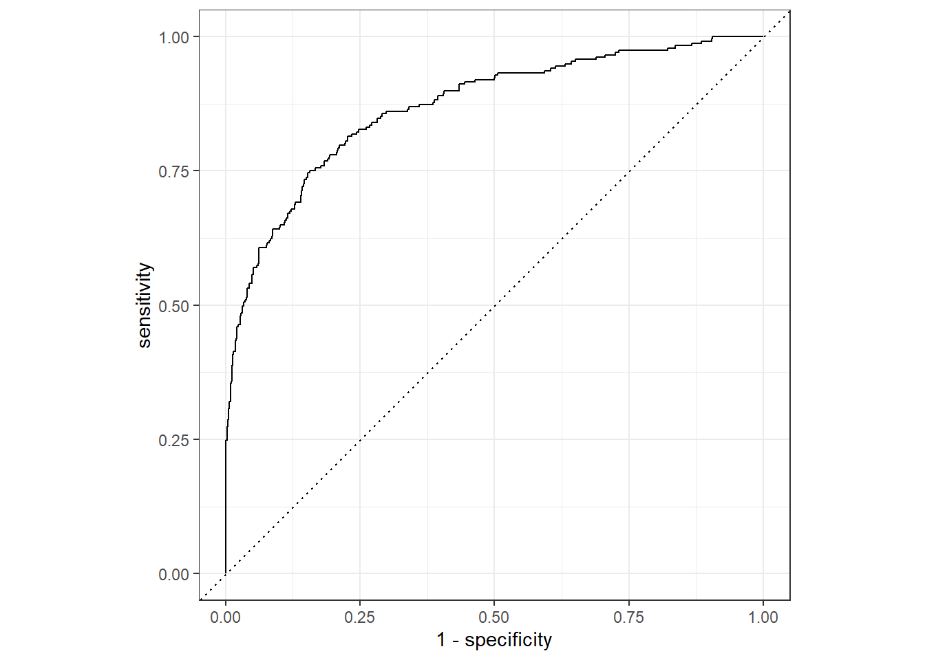
How we use Receiver Operating Curve
Setting the Cross-Validation Scheme using rsample
Rethinking: Why we need validation?
Tidy way to rsample-ing your dataset
rsample is part of tidymodels that could help us in splitting or resampling or machine learning dataset.
There are so many splitting and resampling approach provided by rsample–as you could see in its full function references page. In this introduction, we will use two most general function:
initial_split(): Simple train and test splitting.vfold_cv(): k-fold splitting, with optional repetition argument.
Initial splitting
Initial random sampling for splitting train and test could be done using initial_split():
|
|
#> # A tibble: 1,176 × 35
#>    attrition   age business_travel   daily_rate department    distance_from_home
#>    <chr>     <dbl> <chr>                  <dbl> <chr>                      <dbl>
#>  1 no           53 travel_rarely            238 sales                          1
#>  2 no           28 non_travel              1103 research_dev…                 16
#>  3 no           28 travel_rarely            736 sales                         26
#>  4 no           25 travel_rarely            949 research_dev…                  1
#>  5 no           51 travel_frequently        237 sales                          9
#>  6 yes          32 non_travel              1474 sales                         11
#>  7 no           34 travel_frequently       1003 research_dev…                  2
#>  8 no           40 travel_frequently        593 research_dev…                  9
#>  9 no           36 travel_rarely            884 sales                          1
#> 10 no           27 travel_rarely           1167 research_dev…                  4
#> # ℹ 1,166 more rows
#> # ℹ 29 more variables: education <dbl>, education_field <chr>,
#> #   employee_count <dbl>, employee_number <dbl>,
#> #   environment_satisfaction <dbl>, gender <chr>, hourly_rate <dbl>,
#> #   job_involvement <dbl>, job_level <dbl>, job_role <chr>,
#> #   job_satisfaction <dbl>, marital_status <chr>, monthly_income <dbl>,
#> #   monthly_rate <dbl>, num_companies_worked <dbl>, over_18 <chr>, …
|
|
#> # A tibble: 294 × 35
#>    attrition   age business_travel   daily_rate department    distance_from_home
#>    <chr>     <dbl> <chr>                  <dbl> <chr>                      <dbl>
#>  1 no           27 travel_rarely            591 research_dev…                  2
#>  2 no           59 travel_rarely           1324 research_dev…                  3
#>  3 no           38 travel_frequently        216 research_dev…                 23
#>  4 no           34 travel_rarely           1346 research_dev…                 19
#>  5 yes          36 travel_rarely           1218 sales                          9
#>  6 yes          34 travel_rarely            699 research_dev…                  6
#>  7 no           30 travel_rarely            125 research_dev…                  9
#>  8 no           36 travel_rarely            852 research_dev…                  5
#>  9 no           33 travel_frequently       1141 sales                          1
#> 10 no           27 travel_frequently        994 sales                          8
#> # ℹ 284 more rows
#> # ℹ 29 more variables: education <dbl>, education_field <chr>,
#> #   employee_count <dbl>, employee_number <dbl>,
#> #   environment_satisfaction <dbl>, gender <chr>, hourly_rate <dbl>,
#> #   job_involvement <dbl>, job_level <dbl>, job_role <chr>,
#> #   job_satisfaction <dbl>, marital_status <chr>, monthly_income <dbl>,
#> #   monthly_rate <dbl>, num_companies_worked <dbl>, over_18 <chr>, …
But sometimes, simple random sampling is not enough:
|
|
#>
#>        no       yes
#> 0.8387755 0.1612245
|
|
#>
#>        no       yes
#> 0.8469388 0.1530612
|
|
#>
#>        no       yes
#> 0.8061224 0.1938776
This is where we need strata argument to use stratified random sampling:
|
|
#>
#>        no       yes
#> 0.8387755 0.1612245
|
|
#>
#>        no       yes
#> 0.8391489 0.1608511
|
|
#>
#>        no       yes
#> 0.8372881 0.1627119
Cross-sectional resampling
To use k-fold validation splits–and optionally, with repetition–we could use vfold_cv():
|
|
#> #  3-fold cross-validation repeated 2 times using stratification
#> # A tibble: 6 × 3
#>   splits            id      id2
#>   <list>            <chr>   <chr>
#> 1 <split [980/490]> Repeat1 Fold1
#> 2 <split [980/490]> Repeat1 Fold2
#> 3 <split [980/490]> Repeat1 Fold3
#> 4 <split [980/490]> Repeat2 Fold1
#> 5 <split [980/490]> Repeat2 Fold2
#> 6 <split [980/490]> Repeat2 Fold3
Each train and test dataset are stored in splits column. We could use analysis() and assessment() to get the train and test dataset, consecutively:
|
|
#> # A tibble: 980 × 35
#>    attrition   age business_travel   daily_rate department    distance_from_home
#>    <chr>     <dbl> <chr>                  <dbl> <chr>                      <dbl>
#>  1 yes          41 travel_rarely           1102 sales                          1
#>  2 no           49 travel_frequently        279 research_dev…                  8
#>  3 no           27 travel_rarely            591 research_dev…                  2
#>  4 no           59 travel_rarely           1324 research_dev…                  3
#>  5 no           36 travel_rarely           1299 research_dev…                 27
#>  6 no           35 travel_rarely            809 research_dev…                 16
#>  7 no           29 travel_rarely            153 research_dev…                 15
#>  8 no           31 travel_rarely            670 research_dev…                 26
#>  9 no           34 travel_rarely           1346 research_dev…                 19
#> 10 yes          28 travel_rarely            103 research_dev…                 24
#> # ℹ 970 more rows
#> # ℹ 29 more variables: education <dbl>, education_field <chr>,
#> #   employee_count <dbl>, employee_number <dbl>,
#> #   environment_satisfaction <dbl>, gender <chr>, hourly_rate <dbl>,
#> #   job_involvement <dbl>, job_level <dbl>, job_role <chr>,
#> #   job_satisfaction <dbl>, marital_status <chr>, monthly_income <dbl>,
#> #   monthly_rate <dbl>, num_companies_worked <dbl>, over_18 <chr>, …
|
|
#> # A tibble: 490 × 35
#>    attrition   age business_travel   daily_rate department    distance_from_home
#>    <chr>     <dbl> <chr>                  <dbl> <chr>                      <dbl>
#>  1 yes          37 travel_rarely           1373 research_dev…                  2
#>  2 no           33 travel_frequently       1392 research_dev…                  3
#>  3 no           32 travel_frequently       1005 research_dev…                  2
#>  4 no           30 travel_rarely           1358 research_dev…                 24
#>  5 no           38 travel_frequently        216 research_dev…                 23
#>  6 no           29 travel_rarely           1389 research_dev…                 21
#>  7 yes          34 travel_rarely            699 research_dev…                  6
#>  8 no           44 travel_rarely           1459 research_dev…                 10
#>  9 yes          24 travel_rarely            813 research_dev…                  1
#> 10 yes          50 travel_rarely            869 sales                          3
#> # ℹ 480 more rows
#> # ℹ 29 more variables: education <dbl>, education_field <chr>,
#> #   employee_count <dbl>, employee_number <dbl>,
#> #   environment_satisfaction <dbl>, gender <chr>, hourly_rate <dbl>,
#> #   job_involvement <dbl>, job_level <dbl>, job_role <chr>,
#> #   job_satisfaction <dbl>, marital_status <chr>, monthly_income <dbl>,
#> #   monthly_rate <dbl>, num_companies_worked <dbl>, over_18 <chr>, …
Data Preprocess using recipes
Rethinking: How do we should treat train and test?
Reproducible preprocess recipes
recipes is part of tidymodels that could help us in making a reproducible data preprocess.
There are so many data preprocess approach provided by recipes–as you could see in its full function references page . In this introduction, we will use several preprocess steps related to our example dataset.
There are several steps that we could apply to our dataset–some are very fundamental and sometimes mandatory, but some are also tuneable:
step_rm(): Manually remove unused columns.step_nzv(): Automatically filter near-zero varianced columns.step_string2factor(): Manually convert tofactorcolumns. Downsampling step to balancing target’s class distribution (tuneable).step_center(): Normalize the mean ofnumericcolumn(s) to zero (tuneable).step_scale(): Normalize the standard deviation ofnumericcolumn(s) to one (tuneable).step_pca(): Shrinknumericcolumn(s) to several PCA components (tuneable).
Designing your first preprocess recipes
- Initiate a recipe using
recipe()- Define your formula in the first argument.
- Supply a template dataset in
dataargument.
- Pipe to every needed
step_*()–always remember to put every step in proper consecutive manner. - After finished with every needed
step_*(), pipe toprep()function to train your recipe- It will automatically convert all
charactercolumns tofactor; - If you used
step_string2factor(), don’t forget to specifystrings_as_factors = FALSE - It will train the recipe to the specified dataset in the
recipe()’sdataargument; - If you want to train to other dataset, you can supply the new dataset to
trainingargument, and set thefreshargument toTRUE
- It will automatically convert all
Let’s see an example of defining a recipe:
|
|
#> Recipe
#>
#> Inputs:
#>
#>       role #variables
#>    outcome          1
#>  predictor         34
#>
#> Training data contained 1175 data points and no missing data.
#>
#> Operations:
#>
#> Variables removed employee_count, employee_number [trained]
#> Sparse, unbalanced variable filter removed over_18, standard_hours [trained]
#> Factor variables from business_travel, department, education_field, g... [trained]
#> Factor variables from attrition [trained]
#> Down-sampling based on attrition [trained]
#> Centering for age, daily_rate, distance_from_home, education,... [trained]
#> Scaling for age, daily_rate, distance_from_home, education,... [trained]
#> PCA extraction with age, daily_rate, distance_from_home, education, ... [trained]
There are two ways of obtaining the result from our recipe:
-
juice(): Extract preprocessed dataset fromprep()-ed recipe. Normally, we will use this function to get preprocessed train dataset. -
bake(): Apply a recipe to new dataset. Normally, we use we will use this function to preprocess new dataset, such as test dataset, or prediction dataset.
These are some example on how to get preprocessed train and test dataset:
|
|
#> # A tibble: 378 × 22
#>    business_travel department     education_field gender job_role marital_status
#>    <fct>           <fct>          <fct>           <fct>  <fct>    <fct>
#>  1 travel_rarely   sales          life_sciences   female sales_e… single
#>  2 travel_rarely   research_deve… other           male   laborat… single
#>  3 travel_rarely   research_deve… life_sciences   male   laborat… single
#>  4 travel_rarely   sales          life_sciences   male   sales_r… single
#>  5 travel_rarely   sales          technical_degr… male   sales_r… married
#>  6 travel_rarely   research_deve… medical         male   researc… married
#>  7 travel_rarely   research_deve… life_sciences   male   laborat… single
#>  8 travel_rarely   research_deve… technical_degr… female researc… married
#>  9 travel_rarely   research_deve… life_sciences   male   laborat… single
#> 10 travel_rarely   research_deve… technical_degr… male   laborat… single
#> # ℹ 368 more rows
#> # ℹ 16 more variables: over_time <fct>, attrition <fct>, PC01 <dbl>,
#> #   PC02 <dbl>, PC03 <dbl>, PC04 <dbl>, PC05 <dbl>, PC06 <dbl>, PC07 <dbl>,
#> #   PC08 <dbl>, PC09 <dbl>, PC10 <dbl>, PC11 <dbl>, PC12 <dbl>, PC13 <dbl>,
#> #   PC14 <dbl>
|
|
#> # A tibble: 295 × 22
#>    business_travel   department   education_field gender job_role marital_status
#>    <fct>             <fct>        <fct>           <fct>  <fct>    <fct>
#>  1 travel_rarely     research_de… medical         female laborat… married
#>  2 travel_frequently research_de… life_sciences   male   manufac… single
#>  3 travel_rarely     research_de… medical         male   healthc… married
#>  4 non_travel        research_de… medical         male   laborat… divorced
#>  5 travel_rarely     research_de… medical         male   researc… single
#>  6 travel_frequently research_de… life_sciences   female researc… single
#>  7 travel_rarely     research_de… medical         male   laborat… single
#>  8 travel_rarely     research_de… medical         female researc… divorced
#>  9 travel_rarely     sales        marketing       male   sales_r… married
#> 10 travel_rarely     sales        marketing       female sales_r… married
#> # ℹ 285 more rows
#> # ℹ 16 more variables: over_time <fct>, attrition <fct>, PC01 <dbl>,
#> #   PC02 <dbl>, PC03 <dbl>, PC04 <dbl>, PC05 <dbl>, PC06 <dbl>, PC07 <dbl>,
#> #   PC08 <dbl>, PC09 <dbl>, PC10 <dbl>, PC11 <dbl>, PC12 <dbl>, PC13 <dbl>,
#> #   PC14 <dbl>
Model Fitting using parsnip
Rethinking: How many machine learning packages you used?
One vegeta.. I mean package to rule them all: parsnip
parsnip is part of tidymodels that could help us in model fitting and prediction flows.
There are so many models supported by parsnip–as you could see in its full model list . In this introduction, we will use random forest as an example model.
There are two part of defining a model that should be noted:
-
Defining model’s specification: In this part, we need to define the model’s specification, such as
mtryandtreesfor random forest, through model specific functions. For example, you can userand_forest()to define a random forest specification. Make sure to check full model list to see every model and its available arguments. -
Defining model’s engine: In this part, we need to define the model’s engine, which determines the package we will use to fit our model. This part could be done using
set_engine()function. Note that in addition to defining which package we want to use as our engine, we could also passing package specific arguments to this function.
This is an example of defining a random forest model using randomForest::randomForest() as our engine:
|
|
#> Random Forest Model Specification (classification)
#>
#> Main Arguments:
#>   mtry = ncol(data_train) - 2
#>   trees = 500
#>   min_n = 15
#>
#> Computational engine: randomForest
To fit our model, we have two options:
- Formula interface
- X-Y interface
Note that some packages are behaving differently inside formula and x-y interface. For example, randomForest::randomForest() would convert all of our categorical variables into dummy variables in formula interface, but not in x-y interface.
Fit using formula interface using fit() function:
|
|
#> parsnip model object
#>
#>
#> Call:
#>  randomForest(x = maybe_data_frame(x), y = y, ntree = ~500, mtry = min_cols(~ncol(data_train) -      2, x), nodesize = min_rows(~15, x))
#>                Type of random forest: classification
#>                      Number of trees: 500
#> No. of variables tried at each split: 20
#>
#>         OOB estimate of  error rate: 28.31%
#> Confusion matrix:
#>     yes  no class.error
#> yes 141  48   0.2539683
#> no   59 130   0.3121693
Or through x-y interface using fit_xy() function:
|
|
#> parsnip model object
#>
#>
#> Call:
#>  randomForest(x = maybe_data_frame(x), y = y, ntree = ~500, mtry = min_cols(~ncol(data_train) -      2, x), nodesize = min_rows(~15, x))
#>                Type of random forest: classification
#>                      Number of trees: 500
#> No. of variables tried at each split: 20
#>
#>         OOB estimate of  error rate: 29.89%
#> Confusion matrix:
#>     yes  no class.error
#> yes 136  53   0.2804233
#> no   60 129   0.3174603
In this workflow, it should be relatively easy to change the model engine.
Let’s try to fit a same model specification, but now using ranger::ranger():
|
|
#> Random Forest Model Specification (classification)
#>
#> Main Arguments:
#>   mtry = ncol(data_train) - 2
#>   trees = 500
#>   min_n = 15
#>
#> Engine-Specific Arguments:
#>   seed = 100
#>   num.threads = parallel::detectCores()/2
#>   importance = impurity
#>
#> Computational engine: ranger
Now let’s try to fit the model, and see the result:
|
|
#> parsnip model object
#>
#> Ranger result
#>
#> Call:
#>  ranger::ranger(x = maybe_data_frame(x), y = y, mtry = min_cols(~ncol(data_train) -      2, x), num.trees = ~500, min.node.size = min_rows(~15, x),      seed = ~100, num.threads = ~parallel::detectCores()/2, importance = ~"impurity",      verbose = FALSE, probability = TRUE)
#>
#> Type:                             Probability estimation
#> Number of trees:                  500
#> Sample size:                      378
#> Number of independent variables:  21
#> Mtry:                             20
#> Target node size:                 15
#> Variable importance mode:         impurity
#> Splitrule:                        gini
#> OOB prediction error (Brier s.):  0.2088251
Notice that ranger::ranger() doesn’t behave differently between fit() and fit_xy():
|
|
#> parsnip model object
#>
#> Ranger result
#>
#> Call:
#>  ranger::ranger(x = maybe_data_frame(x), y = y, mtry = min_cols(~ncol(data_train) -      2, x), num.trees = ~500, min.node.size = min_rows(~15, x),      seed = ~100, num.threads = ~parallel::detectCores()/2, importance = ~"impurity",      verbose = FALSE, probability = TRUE)
#>
#> Type:                             Probability estimation
#> Number of trees:                  500
#> Sample size:                      378
#> Number of independent variables:  21
#> Mtry:                             20
#> Target node size:                 15
#> Variable importance mode:         impurity
#> Splitrule:                        gini
#> OOB prediction error (Brier s.):  0.2088251
To get the prediction, we could use predict() as usual–but note that it would return a tidied tibble instead of a vector, as in type = "class" cases, or a raw data.frame, as in type = "prob" cases.
In this way, the prediction results would be very convenient for further usage, such as simple recombining with the original dataset:
|
|
#> # A tibble: 295 × 4
#>    attrition .pred_class .pred_yes .pred_no
#>    <fct>     <fct>           <dbl>    <dbl>
#>  1 no        no              0.336    0.664
#>  2 no        no              0.161    0.839
#>  3 no        no              0.232    0.768
#>  4 no        yes             0.699    0.301
#>  5 yes       no              0.472    0.528
#>  6 yes       yes             0.635    0.365
#>  7 no        yes             0.542    0.458
#>  8 no        no              0.330    0.670
#>  9 yes       yes             0.790    0.210
#> 10 no        yes             0.553    0.447
#> # ℹ 285 more rows
Model Evaluation using yardstick
Rethinking: How do we measure the goodness of our model?
It’s always good to bring your own yardstick
yardstick is part of tidymodels that could help us in calculating model performance metrics.
There are so many metrics available by yardstick–as you could see in its full function references page . In this introduction, we will calculate some model performance metrics for classification task as an example.
There are two ways of calculating model performance metrics, which differ in its input and output:
tibbleapproach: We pass a dataset containing thetruthandestimateto the function, and it will return atibblecontaining the results, e.g.,precision()function.vectorapproach: We pass a vector as thetruthand a vector as theestimateto the function, and it will return avectorwhich show the results, e.g.,precision_vec()function.
Note that some function, like conf_mat() , only accept tibble approach, since it is not returned a vector of length one.
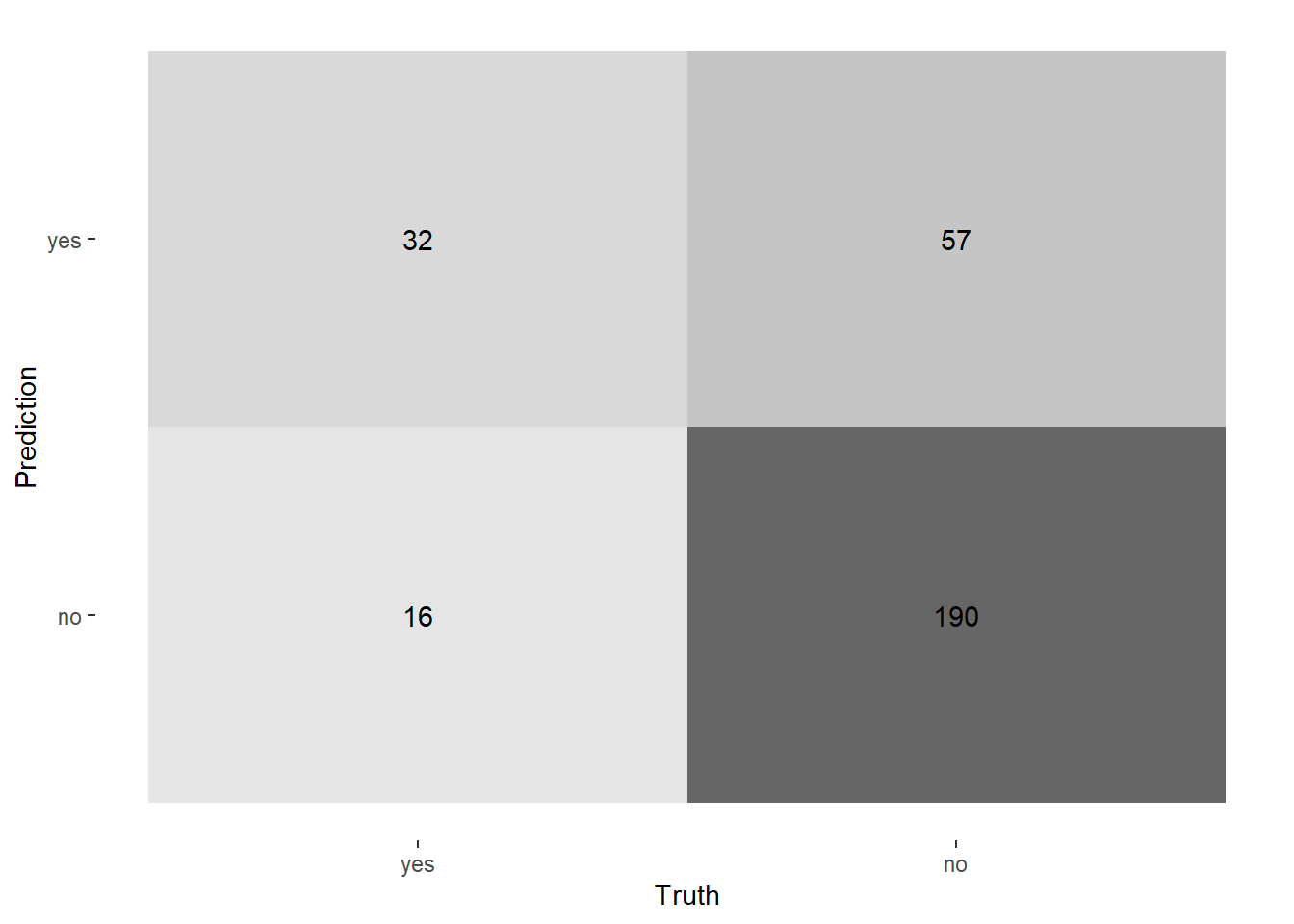
Let’s start by reporting the confusion matrix:
|
|
Now, to calculate the performance metrics, let’s try to use the tibble approach–which also support group_by:
|
|
#> # A tibble: 1 × 3
#>   .metric  .estimator .estimate
#>   <chr>    <chr>          <dbl>
#> 1 accuracy binary         0.753
|
|
#> # A tibble: 3 × 4
#>   department           .metric  .estimator .estimate
#>   <fct>                <chr>    <chr>          <dbl>
#> 1 human_resources      accuracy binary         0.8
#> 2 research_development accuracy binary         0.790
#> 3 sales                accuracy binary         0.677
Or using vector approach, which is more flexible in general:
|
|
#> # A tibble: 1 × 4
#>   accuracy sensitivity specificity precision
#>      <dbl>       <dbl>       <dbl>     <dbl>
#> 1    0.753       0.667       0.769     0.360
|
|
#> # A tibble: 3 × 5
#>   department           accuracy sensitivity specificity precision
#>   <fct>                   <dbl>       <dbl>       <dbl>     <dbl>
#> 1 human_resources         0.8         0.5         0.909     0.667
#> 2 research_development    0.790       0.609       0.816     0.326
#> 3 sales                   0.677       0.762       0.654     0.372
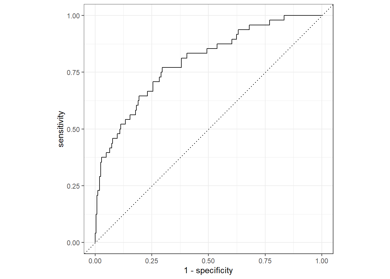
Sometimes the model performance metrics could also improving the models final results. For example, through Receiver Operating Curve, we could assess the probability threshold effect to sensitivity and specificity:
|
|
And, since it’s returning a tibble, we could do further data wrangling to help us see it more clearly:
|
|
#> # A tibble: 297 × 3
#>    .threshold specificity sensitivity
#>         <dbl>       <dbl>       <dbl>
#>  1  -Inf          0                 1
#>  2     0.0546     0                 1
#>  3     0.0699     0.00405           1
#>  4     0.0946     0.00810           1
#>  5     0.103      0.0121            1
#>  6     0.106      0.0162            1
#>  7     0.112      0.0202            1
#>  8     0.120      0.0243            1
#>  9     0.123      0.0283            1
#> 10     0.128      0.0324            1
#> # ℹ 287 more rows
With some ggplot2:
|
|
and plotly magic, it would be perfect:
|
|